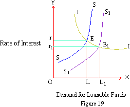
In figure 19, SS and II are the initial savings and investment curves respectively. The point of intersection of these curves is E which represents the initial equilibrium position. At point E the rate of interest is r and amount of savings equal to investment is L. When consumers decide to spend less their unspent portion of the income results in an increased level of savings. This has been shown by a shift in the supply curve of savings from SS to S₁S₁. With increased amount of savings, the rate of interest starts reducing. It falls from r to r₁. With reduction in the rate of interest, the price paid for borrowed loanable funds reduces. This induces producers to invest more to reach a new point of equilibrium E₁. This is a point at which S₁S₁, the saving supply curve intersects the investment demand curve. Once again savings are equal to investment at higher level of loanable funds L₁. Therefore in the new equilibrium position a fall in the rate of interest causes a rise in the amount of investment of the size L₁. This compensates for the fall in the consumption demand for goods and services. As a result of such an increase in the investment demand, the level of aggregate demand is restored. Any danger of large-scale unemployment has thus been avoided. The classical economists have also depended on similar adjustments in the level of prices and wage rates. Hence flexible rates of interest, prices and wage rates together ensure full employment in the loanable funds, commodity and labor markets. Such a self-equilibrating process prevents any dangers of prolonged and general unemployment conditions. 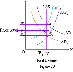The total equilibrium has been shown below in figure 20.

(E) Full Equilibrium: The classical flexible interest, price, wage rate solution automatically leads the economy back to the full employment level. Therefore the effect of a fall in consumer demand on the levels of output and employment is only temporary. In figure 20, AD₁ and SAS₁ are original aggregate demand and aggregate supply curves respectively. The two curves have intersected at point E.

In this equilibrium position original price level is P and real output or national income level is Y. This is full employment equilibrium since the long run supply curve LAS passes through this point. When the consumers reduce their demand for consumption goods the aggregate demand curve then shifts as AD₂. The new AD₂ curve and original SAS₁ curve have intersected at point E1 which is a short run partial equilibrium condition. At E₁ the price level falls to P₁ and real output level reduces to Y₁. Thus a fall in the real output causes some unemployment of labor and other resources. But due to equilibrating forces at work, such as a fall in the rate of interest and a cut in the wage rates, a fresh demand for investment goods is generated. A fall in the wage rates reduces cost of production which induces producers to employ more workers. As a result of these adjustments the economy moves from E₁ to a new equilibrium point E₂. At this point AD₂ intersects the new supply curve SAS₂ which has shifted downwards. Such a shift in the supply curve shows a fall in the cost of production due to a cut in the wage rates. At point E₂ the original equilibrium level of output Y can be produced which is the full employment level of output. The price level has now fallen to P₂. Thus with a fall in the rate of interest, price level and wage rate, the restoration of full employment equilibrium level becomes possible.

[next page]

Index

5. 1 Classical Theory
5. 2 Keynes' Employment Theory

Chapter 6