|
4.3 Equilibrium
Given the supply and demand curves in their aggregate form, an equilibrium level can be established at the point of their intersection.
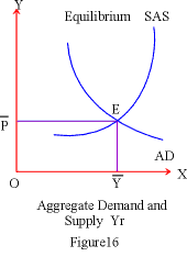
In figure 16, AD and SAS are such short run curves. The two have intersected at point E which is the equilibrium; the price that is commonly offered and received is P and quantity exchanged is Y (P and Y bar). This is only an initial equilibrium and it can alter with a shift in either the demand or supply curves.
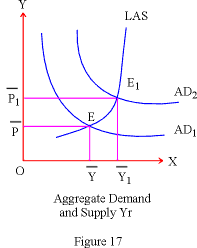
In figure 17 such a shift upwards in the aggregate demand curve has been shown. This causes equilibrium position to shift as well from E to E1. In the new equilibrium position price level rises from P to P1 and real output quantity exchanged increases from Y to Y1. Such an increase in the real output becomes possible because between E and E1 we were still operating along the short run supply phase, where some resources were underutilized. But once the point E1 is reached the supply curve becomes steep and vertical. Here the full employment level is reached and no more resources are available for further additions to be made to the real output. Therefore E1Y1 is a vertical full employment long run supply curve (LAS). Points such as E are partial equilibrium under employable points.
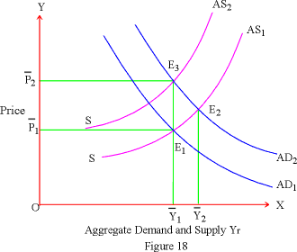
Finally in figure 18 we have an interesting case where aggregate demand shifts and increases beyond full employment level. In this case E1 is the original point of equilibrium with AD1 and SAS1 having intersected at this point. However this happens to be the full employment condition and LAS passes through this point which is Y1E1. If aggregate demand further shifts upwards as shown by AD2 then a new point of equilibrium is attained at E2 where AD2 and SAS1 have intersected. The new price level is then P2 and output quantity Y2 . However, since all available resources were fully employed and exhausted at Y output level, this increase is purely a monetary phenomenon caused by rising price level. Therefore movement from Y1 to Y2 is only an increase in money value of the real output. This becomes possible because contracted agents of production have secured a hike in their wages, rent and interests. As a result of increase in input prices and consequent rise in the cost of production, the supply curve shifts upwards as SAS2. Yet another point of intersection between AD2 and SAS2 becomes possible at a new equilibrium level E3. In this equilibrium position we revert to the old full employment level of output Y1though the price level is now higher than before as P2. Thus in the long run after all adjustments have taken place the economy settles down at the full employment level and only price level rises upwards due to inflationary pressure.
**********
|