|
11.2 Monopoly Demand Curve
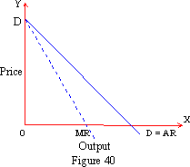
(A) Downward Sloping Curve D: In case of a competitive firm, price is given and fixed. Demand or Average Revenue curve is perfectly flexible and is a horizontal straight line. A monopolist has the freedom to charge a higher or lower price. With a change in the price, the quantity demanded also alters. Again a monopolist is a single seller. He himself is a firm as well as an industry. Hence market demand curve is in itself the demand curve of the monopolist. As a result of this the demand curve of a monopolist is downward sloping.

This has been shown in Figure 40. DD in the figure is the Demand or Average Revenue curve of a monopolist. When the Average Revenue curve falls, the corresponding Marginal Revenue curve also falls and is below the AR curve. The usual law about the behavior of average and marginal quantities governs such a relation between AR and MR.
(B) AR-MR Relationship: The relation between Average and Marginal Revenue is similar to that of the behavior of average and marginal quantities in general, such as costs, wages etc. When the marginal quantity is constant, average quantity is also constant and the two values are identical. When the marginal quantity increases, the average quantity likewise increases and is lower than the marginal quantity. On the other hand, when the marginal quantity decreases the average quantity falls but is above or greater than the marginal value. This has been illustrated in the table below.
Click to view the Table
The table makes the MR-AR relationship clear. In part I where total quantity increases from 10 to 20 to 30 marginal quantity remains constant at 10 (20 -10 = 10, 30 - 20 = 10). Average quantity is also constant and equal to 10 (20 ¸ 2 = 10, 30 ¸ 3 = 10). When the marginal quantity increases as 10, 15, 20 though the average quantity increases it is smaller in value and is below the marginal quantity. When the marginal value falls as 10, 8, 6 the average value also tends to fall as 10, 9, 8. In this case, average value is more than and above marginal value. This has further been made clear with an arrow diagram in Figure 41.

Here A the average quantity and M the marginal quantity are equal when the two are constant. When A rises, M1 is above A and when A falls, M2 is below A. This relationship is applicable to all forms of markets and for all average marginal quantities. The reason for such behavior is simple. It is Marginal Change which makes the average quantity behave one way or the other. Marginal Change is a single unit change whereas average value gets distributed over all previous units. When M increases from 10 to 15, 5 is added to M. This value is distributed over two units to produce Average Change of 5 ¸ 2 = 2.5; hence the rise from 10 to 12.5.
[next page]
|