8.7 Critical Region
Now  i.e. the relative deviation of sample is a standard normal variate
from which it is extremely useful to draw statistical inference. i.e. the relative deviation of sample is a standard normal variate
from which it is extremely useful to draw statistical inference.
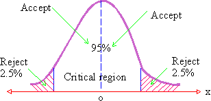
We know that the standard normal variate is our z - score. 95% area under the curve lies between -1.96 and +1.96, 99% lies between -2.58 and +2.58 and 99.73% lies between -3 and +3. In other words, only 5% area under the normal curve lies beyond ± 1.96, 1% , beyond ± 2.58 and 0.27% lies beyond ±3. These areas also indicate the probabilities that the z - score exceeds these values i.e. the probability that z - score will exceed 1.96 numerically is 0.05.
\ P ( z < -1.96 or z > 1.96 ) = 0.05
\ P ( | z | > 1.96 ) = 0.05
This means that the probability that z - score will lie in the shaded region is 0.05 which is very small.
Similarly P ( | z | > 2.58 ) = 0.01 and P P ( | z | > 3 ) = 0.0027.
Return to our z - score formula  where mean of sample is for which z-score is z1 . where mean of sample is for which z-score is z1 .
Now 95 out of 100 values of z1 will lie between
-1.96 and +1.96. For z1 > 1.96 or z1 <
1.96 , a rare event has taken place because p ( | z1
| > 1.96 ) = 0.05 which is very small. The z - score (z1
of x1 from m0 is
so significant that it can not due to sample fluctuations alone.
If p ( | z1 | > 2.58 ) = 0.01, then very unusual event has taken place because this probability is extremely small (remote). Again we can firmly say that the deviation of x1 from m0 (i.e. z - score ) is significant and it is not due to the sample fluctuations alone.
From this discussion we come to a strong conclusion that the levels marked by the probabilities 0.05 or 0.01 which determine the significance of an event are called Levels Of Significance and are always expressed in percentages as 5% level of significance or 1% level of significance. The corresponding regions are called Critical Regions.

The limits within which we expect z-score lies with specified probabilities are called 'Confidence limits'. Thus p ( | z | > 1.96 ) = 0.05 and the bounding values are ± 1.96 are the confidence limits or fiducial limits. It means we are confident that 95 cases out of 100, the sample mean x will be such that z lies between -1.96 and +1.96.
Main objects of sampling theory are (i) Estimation (ii) Testing a hypothesis.
|